Formulas
Excel Tutorial
Excel is great for working with numbers and math. Sometimes you do that by entering formulas, and in this course you'll learn how to add, subtract divide, and multiply by typing formulas into Excel worksheets.
You'll also learn how to use simple formulas that automatically update their results when values change. If you need to revise a value after a total is calculated, no problem. Just make the change, and Excel updates the total for you.
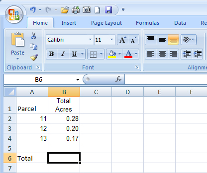
Imagine that Excel is open and you're looking at the Total Acres column. Cell B6 in the worksheet is empty; the amount of total acreage hasn't been entered yet.
In this lesson you'll learn how to use Excel to do basic math by typing simple formulas into cells. You'll also learn how to total all the values in a column with a formula that updates its result if values change later on.
The three separate acreage amounts are .28, .20 and .17. The total of these three values is the total acreage under consideration.
You can add these values in Excel by typing a simple formula into cell B6.
Excel formulas always begin with an equal sign (=). Here's the formula typed into cell C6 to add .28, .20 and .17:
=.28+.20+.17
The plus sign (+) is a math operator that tells Excel to add the values.
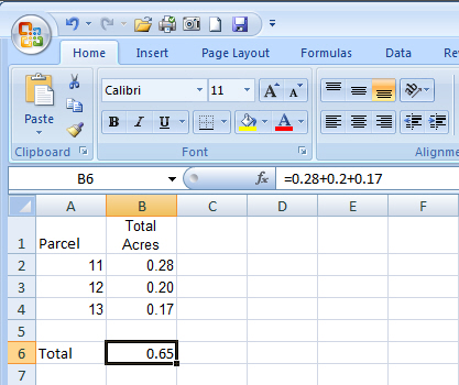
If you wonder later on how you got this result, the formula is visible in the formula bar![]() near the top of the worksheet whenever you click in cell B6 again.
near the top of the worksheet whenever you click in cell B6 again.
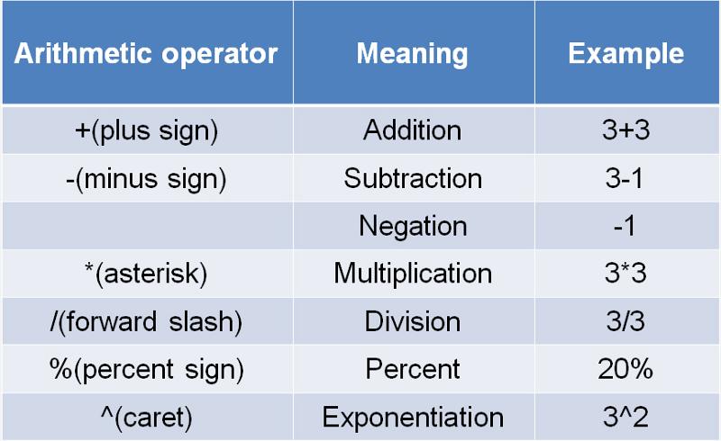
To do more than add, use other math operators as you type formulas into worksheet cells.
Use a minus sign (-) to subtract, an asterisk (*) to multiply, and a forward slash (/) to divide. Remember to always start each formula with an equal sign.
Note You could use more than one math operator in a single formula. This course covers only single-operator formulas, but you should know that if there's more than one operator; formulas are not just calculated from left to right.
Another method of calculating the total acreage is to use a prewritten formula, called a function.
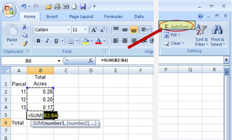
You can get the total in cell B5 by clicking Sum![]() in the Editing group on the Home tab. This enters the SUM function, which adds up all the values in a range of cells. To save time, use this function whenever you have more than a few values to add up, so that you don't have to type the formula.
in the Editing group on the Home tab. This enters the SUM function, which adds up all the values in a range of cells. To save time, use this function whenever you have more than a few values to add up, so that you don't have to type the formula.
Pressing ENTER displays the SUM function result .65 in cell B5. The formula =SUM (B2:B4) appears in the formula bar whenever you click in cell B5.
B2:B4 is the information, called the argument, which tells the SUM function what to add. By using a cell reference (B2:B4) instead of the values in those cells, Excel can automatically update results if values change later on. The colon (:) in B2:B4 indicates a cell range in column B, rows 2 through 4. The parentheses are required to separate the argument from the function.
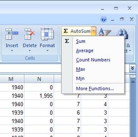
Several of the most common summary statistics can be found on the drop down menu under AutoSum. Any of these can be used by moving to the cell below the last data item in any column, selecting the drop down item and hitting enter. Sum will calculate the total value of all numeric entries; Average will calculate the mean value of those same entries; Count Numbers will calculate the number of numeric entries; Max will calculate the largest numeric entry; and Min will calculate the smallest numeric entry.
Tip The Sum button is also on the Formulas tab. You can work with formulas no matter what tab you work on. You might switch to the Formulas tab to work with more complex formulas.
Tip: Especially for large worksheets, you will find it useful to have the column headings visible at all times. One way to accomplish this is to select the Freeze Panes option under the View tab and then select Freeze Top Row. It can be unfrozen at any time.
Sometimes it's easier to copy formulas than to create new ones. In this example, you'll see how to copy the formula used to get the total of all selling prices and use it to add up the Total Cost Values.
First you select cell E103, which contains the sum of the Sale Prices formula. Then, position the mouse pointer over the lower-right corner of the cell until the black cross (+) appears. Next, drag the fill handle![]() over cell F103. When the fill handle is released, the Total Cost Values total appears in cell F103. The formula =SUM (F2:F102) is visible in the formula bar near the top of the worksheet whenever you click in cell F103.
over cell F103. When the fill handle is released, the Total Cost Values total appears in cell F103. The formula =SUM (F2:F102) is visible in the formula bar near the top of the worksheet whenever you click in cell F103.
Notice also that cell F103 may be filled with " # ". That is because there is insufficient width to display the answer. Column widths can be adjusted manually by clicking on the right vertical border and dragging it. Excel will also automatically adjust to the widest entry when the user double clicks on the column boundary.
After the formula is copied, the Auto Fill Options button ![]() appears to give you some formatting options. In this case you wouldn't need to do anything with the button options. The button disappears when you next make an entry in any cell.
appears to give you some formatting options. In this case you wouldn't need to do anything with the button options. The button disappears when you next make an entry in any cell.
Play this movie to see how a formula is copied.
Note You can drag the fill handle to copy formulas only into cells that are next to each other, either horizontally or vertically.
Cell references identify individual cells in a worksheet. They tell Excel where to look for values to use in a formula.
Excel uses a reference style called A1, which refers to columns with letters and to rows with numbers. The letters and numbers are called row and column headings.
In this lesson you'll see why Excel can automatically update the results of formulas that use cell references, and how cell references work when you copy formulas.
What happens if the value in a cell changes after a total is calculated?
Suppose it turned out that the 0.17 value in cell B4 under Total Acres was incorrect. It was actually 0.19 acres instead. You change that amont in one of the ways described previously and hit ENTER.
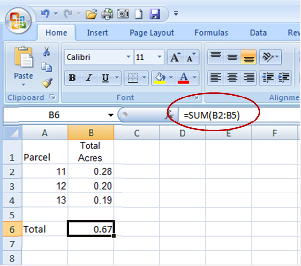
As the picture shows, when the value in cell B4 changes, Excel automatically updates the total in cell B6 from 0.65 to 0.67. Excel can do this because the original formula =SUM (B2:B4) in cell B6 contains cell references.
If you had entered specific values into a formula in cell B6, Excel would not be able to update the total. You'd have to change not only the figures in cell B4, but in the formula in cell B6 as well.
Note You can revise a formula in a selected cell by typing either in the cell or in the formula bar ![]() .
.
You can type cell references directly into cells, or you can enter cell references by clicking cells, which avoids typing errors.
In the first lesson you saw how to use the SUM function to add all the values in a column. You could also use the SUM function to add just a few values in a column, by selecting the cell references to include.
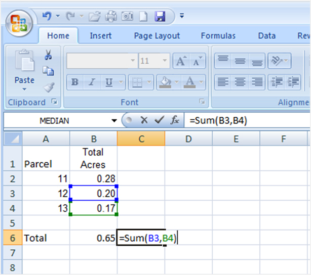
Imagine that you want to know the combined acreage for parcels 12 and 13. You don't need to store the total, so you could enter the formula in an empty cell and delete it later. The example uses cell C6.
The example shows you how to enter the formula. You would click the cells you want to include in the formula instead of typing the cell references. A color marquee surrounds each cell as it is selected and disappears when you press ENTER to display the result 0.37. The formula =SUM (B3, B4) appears in the formula bar near the top of the worksheet whenever cell C6 is selected.
The arguments B3 and B4 tell the SUM function what values to calculate with. The parentheses are required to separate the arguments from the function. The comma, which is also required, separates the arguments.
Now that you've learned more about using cell references, it's time to talk about different types of references:
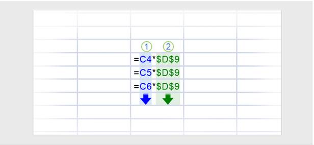
Relative Every relative cell reference in a formula automatically changes when the formula is copied down a column or across a row. This is why you could copy the Sale Price formula to add up Total Cost Values. As the example illustrated here shows, when the formula =C4*$D$9 is copied from row to row, the relative cell references change from C4 to C5 to C6.
Absolute An absolute cell reference is fixed. Absolute references don't change if you copy a formula from one cell to another. Absolute references have dollar signs ($) like this: $D$9. As the art shows, when the formula =C4*$D$9 is copied from row to row, the absolute cell reference remains as $D$9.
Mixed A mixed cell reference has either an absolute column and a relative row, or an absolute row and a relative column. For example, $A1 is an absolute reference to column A and a relative reference to row 1. As a mixed reference is copied from one cell to another, the absolute reference stays the same but the relative reference changes.
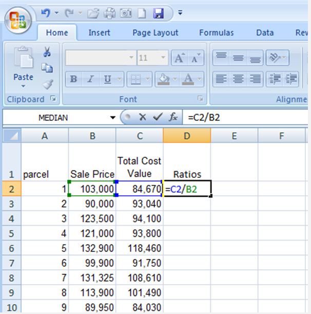
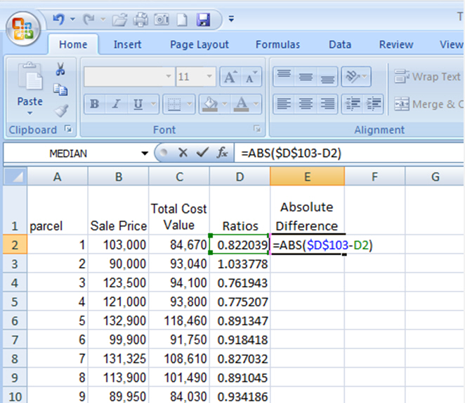
Copy everything in the Parcel, Sale Price and Total Cost Value columns to a separate worksheet. Then enter the formula =C2/B2 in cell D2. You can do that either by typing it directly into D2 or by typing '=' then pointing to C2, typing '/', and finally pointing to B2. The result of 0.822039 should be displayed in D2 after you hit ENTER.
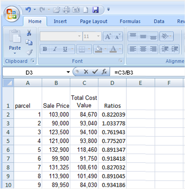
This formula uses relative references. You can see that if you simply copy it to D3. The formula in that cell is now '=C3/B3'.
Copy this formula down the remainder of column D. This can be done by dragging down to the bottom of the column or double clicking the mouse with the cursor at the bottom right corner of cell D3.
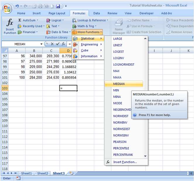
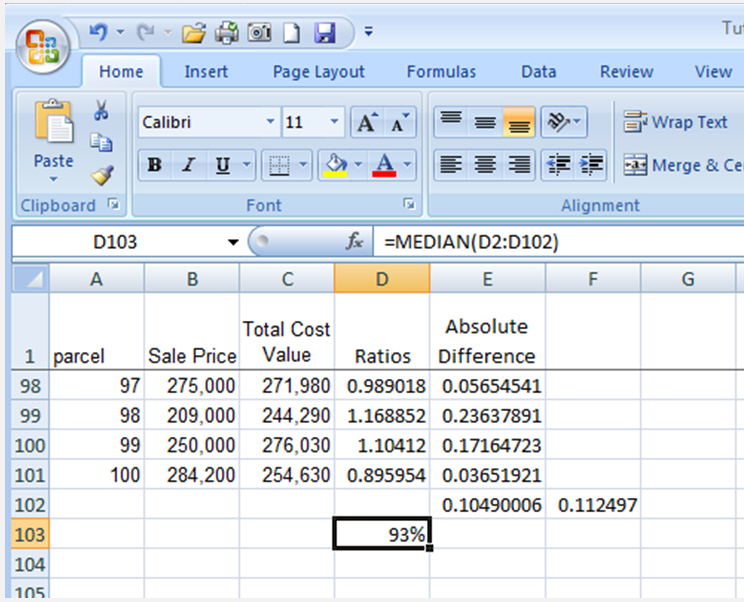
Move beyond the bottom of column D to cell D103. Select the Formulas tab and the More Functions options in the Function Library group. This will cause a drop down menu to appear containing a list of available functions. Move down that list to MEDIAN and select it.
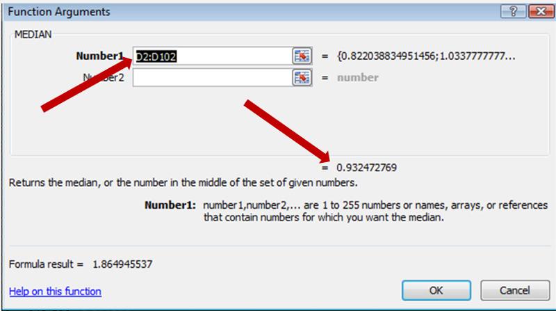
At that point a dialog box should appear in the center of your screen. It will display the arguments D2:D102 in the window labeled Number 1. It will also show the result of calculating the median based on the cells in that range. When you select 'OK', that result will be shown in cell D103.
The formula =MEDIAN (D2:D102) will also appear in the formula window.
Part of the calculation of the coefficient of dispersion (COD) involves finding the absolute difference between every ratio and the median. The Median ratio has been calculated and is found in cell D103. Because we want every calculation to reference that cell, we will make that reference in the formula absolute ($D$103). The reference to each cell containing the ratios can be relative.
SUM is just one of the many Excel functions. These prewritten formulas simplify the process of entering calculations. Using functions, you can easily and quickly create formulas that might be difficult to build for yourself.

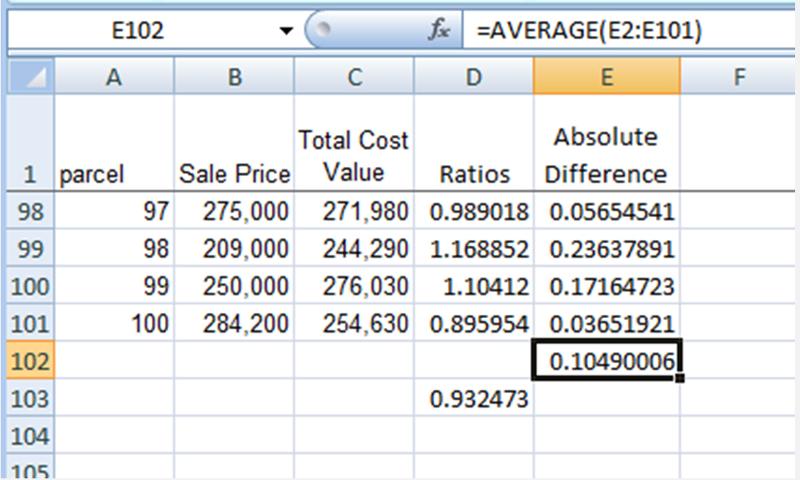
You can use the AVERAGE function to find the average absolute deviation from the median.
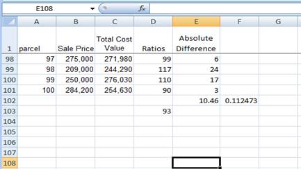
Excel will enter the formula for you. Click in cell E102. On the Home tab, in the Editing group, click the arrow on the Sum button, and click Average in the list. The formula =AVERAGE (D2:D101) appears in the formula bar ![]() near the top of the worksheet. Excel will tend to use the closest cell with a numeric value in it in these functions. If you placed the cursor at E103, Excel would attempt to use D103 as an argument. If you want the average to appear in E103, you should type the formula in that cell instead of using the menu.
near the top of the worksheet. Excel will tend to use the closest cell with a numeric value in it in these functions. If you placed the cursor at E103, Excel would attempt to use D103 as an argument. If you want the average to appear in E103, you should type the formula in that cell instead of using the menu.
The coefficient of dispersion can be easily calculated using the previous results. Move your cursor to an empty cell, say F102 and enter the formula '=E102/D103'.
This is a good place to talk about formatting. There are two ways you as a user may approach formatting. The first involves changing the way numbers are displayed without changing the underlying number. You may select this approach when you want an interim report that does not change the underlying number. The second involves changing the underlying number for both display and further calculation.
The median ratio was calculated as 0.932473. By right clicking on the cell containing the median ratio (D103), a dialog box appears that allows the user to make several different changes. Using the Number tab and selecting Percentage, the user can change the display of the median to a percentage.
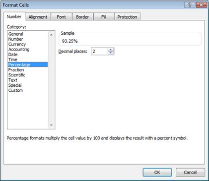
Notice when the decimal places are changed to 0 and we hit OK the median changes to 93%. However, all other figures on the worksheet remain unchanged. That is because only the appearance of the number has changed.
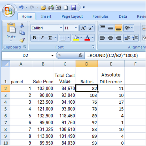
Another approach changes the underlying number. Remember the original formula for the Ratio was '=C2/B2' for the first ratio. We can begin adjusting that formula by multiplying the result by 100. We can show the result in a separate column or revise the existing ratio. Be sure to separate every function in Excel with parentheses. Now the formula becomes '= (C2/B2)*100' and the result is 82.20388 for the first ratio. To represent that ratio as a whole number, we add the Round function to the front of the formula =Round ((and indicate the number of places to round by adding a ',' and a '0'. The final formula appears as "=ROUND((C2/B2),0)". The number of places to round are indicated by the size of the number, to the right is indicated by positive numbers (greater than zero), with the sign assumed, and to the left by negative numbers (less than 0).
=ROUND((C2/B20,0) -> 82
=ROUND((C2/B20,1) -> 82.2
=ROUND((C2/B20,-1) -> 80
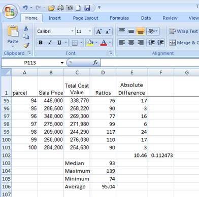
The median ratio will have to be reformatted now so that it doesn't show 9300%. The average absolute deviation has already been rounded along with the ratios.
It is good practice to label calculated results for future reference.
Some of the other summary statistics that might be helpful are shown below.
0
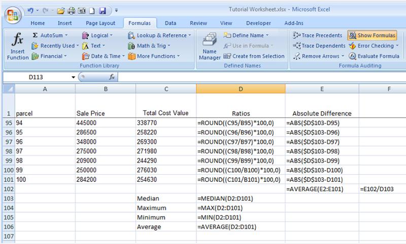
You can print formulas and put them up on your bulletin board to remind you how to create them.
To print formulas, you need to display formulas on the worksheet. You do this by clicking the Formulas tab, and in the Formula Auditing group, clicking Show Formulas![]() .
.
Hide the formulas on the worksheet by repeating the step to display them.
Sometimes Excel can't calculate a formula because the formula contains an error. If that happens, you'll see an error value instead of a result in a cell. Here are three common error values:
# # # # # The column is not wide enough to display the contents of this cell. Increase column width, shrink the contents to fit the column, or apply a different number format.
#REF! A cell reference is not valid. Cells may have been deleted or pasted over.
#NAME? You may have misspelled a function name or used a name that Excel does not recognize. You should know that cells with error values such as #NAME? may display a color triangle. If you click the cell, an error button ![]() appears to give you some error correction options.
appears to give you some error correction options.
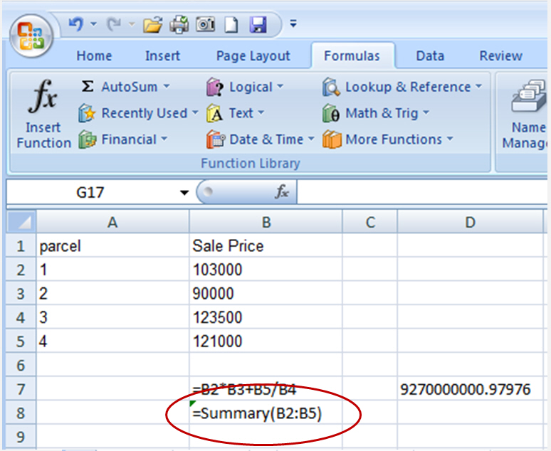
In this case, the user typed Summary, which is not an Excel function.
Excel offers many other useful functions, such as date and time functions and functions you can use to manipulate text.
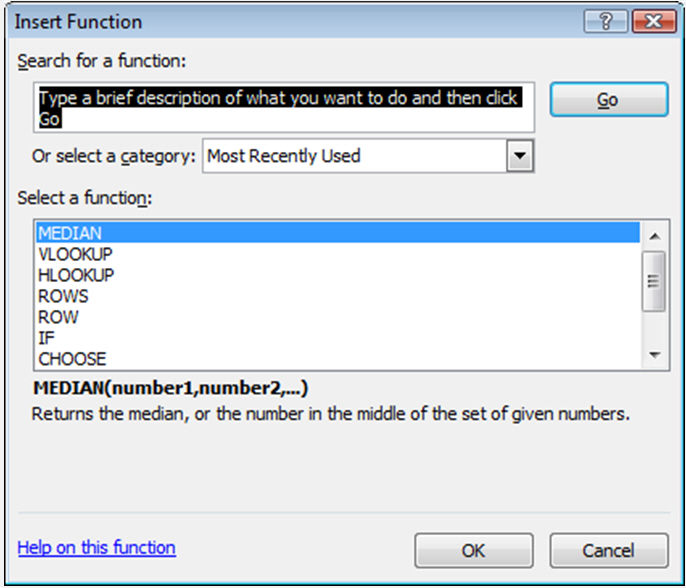
To see all the other functions, click the arrow on the Sum button in the Editing group on the Home tab, and then click More Functions in the list. In the Insert Function dialog box that opens, you can search for a function. This dialog box also gives you another way to enter formulas in Excel. You can also see other functions by clicking the Formulas tab.
With the dialog box open, you can select a category and then scroll through the list of functions in the category. Click Help on this function at the bottom of the dialog box to find out more about any function.